


At a glance
- DEA Water Observations aims to provide consistent, long‑term insight into surface‑water behaviour.
- It maps where surface water has been observed across Australia using Landsat imagery from 1986 to the present.
- An automated algorithm classifies each 30‑m Landsat pixel as wet, dry, or not observable, creating a continent‑scale record of water presence and variability.
- The dataset distinguishes areas with permanent water from those with intermittent or rare inundation, supporting flood analysis, wetland monitoring and water‑resource management.
Background to DEA Water Observations
DEA Water Observations – formerly Water Observations from Space (WOfS) – is a national surface‑water dataset that provides a consistent historical record of where water has been observed across Australia over time.
Using the long‑term Landsat archive (1986–present), the dataset maps surface water across the continent as new imagery becomes available. An automated algorithm classifies each 30‑m Landsat pixel as wet, dry, or not observable, based on water’s distinctive spectral signature and the number of clear, cloud‑free observations.
By summarising decades of imagery from Landsat 5, 7, 8 and 9, DEA Water Observations shows where water is persistent (such as lakes, rivers and dams) and where it occurs only intermittently during floods or temporary inundation.
This long‑term view supports better understanding of flood behaviour, wetland dynamics, water connectivity and interactions between surface water and groundwater.
Using the signature of water
The method relies on the distinct spectral signature of water, particularly its strong absorption of longer wavelengths of light.
For every location, the algorithm compares the number of times water was detected with the total number of clear observations, producing a long‑term record of water presence and variability.
Originally developed by Geoscience Australia as part of the Australian Government’s response to the 2011 floods, it now forms a core product within the National Flood Risk Information Project.
What can we learn from observations of surface water
Understanding through monitoring surface water can help to:
- identify where historical flooding has occurred to help build a clearer picture of flood‑prone areas
- understand how permanent or persistent waterbodies are to help land‑use and infrastructure planning
- support wetland assessments and track how water moves across the landscape, including links between surface water and groundwater systems
- trace year‑to‑year changes in water availability, offering insights that help with drought monitoring and response
- compare seasonal differences in water presence, such as how availability shifts between summer and winter.
The map's two datasets
- In the context of climate change, information from DEA Water Observations can be used to understand existing flood and inundation risk at a location.
- Specifically, when conducting a risk assessment, it is useful to identify any existing risk of flooding or inundation in the coastal area.
- Where there are no local studies, DEA Water Observations can give a broad understanding of the previous flood and inundation history.
For each grid cell (30 m pixel), the DEA Water Observations provide two datasets:
- Water Summary (filtered): this shows the percentage of clear (cloud/shadow‑free) satellite observations classified as water calculated over the full Landsat record (1986–present). Values are masked where Confidence is below 10%, so you see only the more reliable water frequencies
- Confidence: this is the confidence in that data. It expresses, as a percentage, the probability that the water frequency at a pixel reflects real water. It is derived via a logistic‑regression model that considers terrain (e.g. slope, elevation, topographic position), independent satellite indicators of water, mapped water features, and observation frequency.

- In Shoreline Explorer, click the box for DEA water Observations (WOfS)
- If you want to see the local government boundaries also click on this dataset.
- To find your area of interest either: type the name of the place in the search box (top right hand corner of the map), or zoom in using the zoom slider
- Just below the tickbox for WOfS, choose between the two datasets.
You want to look at the actual data - water summary (filtered).
Next look at the confidence in that data. - Use the horizontal slide bar to set your transparency/opacity for the displayed data.
Dataset 1. Water summary (filtered)
When you select this dataset, you will see a coloured map in which different colours show the percentage of clear observations when water was detected. The key on the left shows the interpretation of colours (Figure 1).
For example:
- Red colour at a location indicates only 1% of the observations identified water at that location. This means the location does not have a regular presence of water but may have flooded in the past (1%, if all observations are clear, is 3-4 days per year).
- Blue colour suggests 80% of observations identified water at that location, indicating that the location is a semi-permanent water body.

Figure 1: Example of Dataset 1 Water summary (filtered) in CoastAdapt's depiction of DEA Water Observations.
DEA water observations
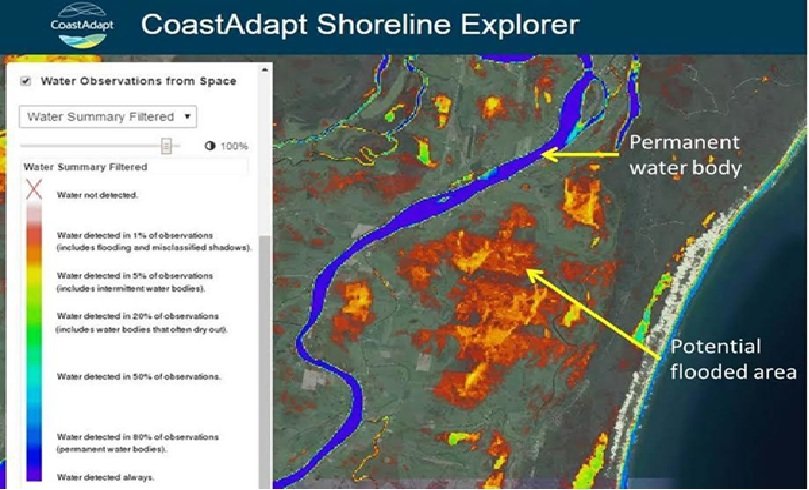
Figure 1: Example of Dataset 1 Water summary (filtered) in CoastAdapt's depiction of DEA Water Observations.
Limitations of Dataset 1 - the water observations
The current limitations of WOfS are:
- Not all floods are captured.
Landsat satellites image a 185‑km‑wide swath and return to the same location roughly every 16 days. This means they only record what was visible on the day of overpass. As a result, many historical floods - especially short‑lived events - may not have been observed.
- Small water bodies can be missed
Although the water‑detection algorithm has a high overall accuracy (≈97%), it is optimised for detecting larger water features, so small or narrow waterbodies may not be consistently detected.
- Mixed water–vegetation pixels can lead to underestimation.
Along rivers, swamps, floodplains, and vegetated wetlands, water may be present beneath vegetation. When water and vegetation occupy the same 30‑m pixel, the algorithm may classify the pixel as dry, underestimating the true extent of water.
- Some steep or urbanised areas may be misclassified.
Highly reflective or complex surfaces, such as dense urban areas or steep terrain, can be misidentified as water due to spectral similarity or shadowing in some landscapes.
Dataset 2. Confidence
Due to the above limitations with dataset 1, WOfS provides a second dataset showing the confidence in the water summary information at each location.
In Figure 2, red indicates low confidence (less than 2%) and green suggest high (75%) to very high (100%) confidence in the information (Figure 2).
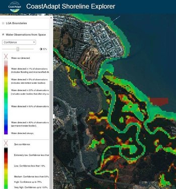
Figure 2. Example of Dataset 2 Confidence in CoastAdapt's DEA Water Observations.
DEA water observations_2

Figure 2. Example of Dataset 2 Confidence in CoastAdapt's DEA Water Observations.
These two datasets can build understanding of past flooding extent at a location. For example, if a location shows red in the Water summary dataset, and green in the Confidence dataset, you can be confident that this indicates a past history of flooding.
more at Geoscience Australia's DEA Water Observations
Keep in mind
- The absence of water observations at a particular location does not provide certainty that flooding will never occur in the future.
- The probability of surface water appearing at a particular location may vary over time due to anthropogenic changes.
- For example, dam construction.
- Where such changes have occurred, Dataset 1 may no longer give a true picture of the probability of surface water being observed.
- Further details on WOfS are available in the product description.
Source
Muller, N., A. Lewis, D. Roberts, S. Ring, R. Melrose, J. Sixsmith, L. Lymburner, A. Mcintyre, P. Tan, S. Curnow and A. IP, 2016: Water observations from space: Mapping surface water from 25 years of Landsat imagery across Australia. Remote Sensing of Environment, 174, 341-352. [http://www.sciencedirect.com/science/article/pii/S0034425715301929].